Overview

RQuantLib connects GNU R with QuantLib.

What is R ?

R is designed as a true computer language with control-flow constructions for iteration and alternation, and it allows users to add additional functionality by defining new functions. For computationally intensive tasks, C, C++ and Fortran code can be linked and called at run time. R is an official part for the GNU Project.

What is QuantLib ?

So what can RQuantLib (currently) do?

So what does RQuantLib (currently) do with Options?

Moreover, another base class ImpliedVolatility is provided with methods print and summary and implied volatility solvers for European and American are provided (Binaries seem to trigger a QuantLib bug as far as I can tell).

For both option and implied volatility calculations, operations are limited to the scalar case. However, using the R, or rather, S object framework makes the work fairly convenient.

Lastly, for the basic European Option, an "array" interface is provided. Here, any of the usual input variables is allow to be in vector form. Solutions are then computed for the "multi-dimensional outer product" of all input vectors. Concretely, if called with three strike prices, four maturities and five volatilities, then 3 * 4 * 5 arrays are returned for the common variables of interest (i.e. value, delta, gamma, ...). In other words, value is now an array over all possible combination of all possible input values. This allows for very compact comparison and scenario analysis.

So what does RQuantLib (currently) do with Fixed Income?

The BermudanSwaption function prices a Bermudan swaption with specified strike and maturity (in years), after calibrating the selected short-rate model to an input swaption volatility matrix. Swaption maturities are in years down the rows, and swap tenors are in years along the columns, in the usual fashion. It is assumed that the Bermudan swaption is exercisable on each reset date of the underlying swaps.

The Fixed Income functions are a good illustration of the R/C++ interface provided by the Rcpp package by Dominick Samperi (available on CRAN as a package of the same name).

What else is there?

Examples

A simple example for EuropeanOption

> library(RQuantLib)
> EO <- EuropeanOption("call", 100, 100, 0.01, 0.03, 0.5, 0.4)
> print(EO)
Concise summary of valuation for EuropeanOption
   value    delta    gamma     vega    theta      rho   divRho
 11.6365   0.5673   0.0138  27.6336 -11.8390  22.5475 -28.3657
> summary(EO)
Detailed summary of valuation for EuropeanOption
   value    delta    gamma     vega    theta      rho   divRho
 11.6365   0.5673   0.0138  27.6336 -11.8390  22.5475 -28.3657
with parameters
         type    underlying        strike dividendYield  riskFreeRate
       "call"         "100"         "100"        "0.01"        "0.03"
     maturity    volatility
        "0.5"         "0.4"

A simple example for EuropeanOptionImpliedVolatility

> EOImpVol <- EuropeanOptionImpliedVolatility("call", value=EO$value+0.50, 100, 100, 0.01, 0.03, 0.5, 0.4)
> print(EOImpVol)
Implied Volatility for EuropeanOptionImpliedVolatility is 0.418
> EOImpVol$impliedVol
[1] 0.4181017

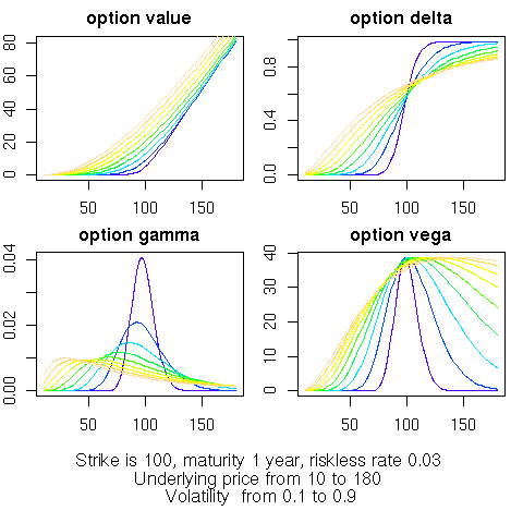
An example of the array-style access

> example(EuropeanOptionArrays)

ErpnOA> und.seq <- seq(10, 180, by = 5)

ErpnOA> vol.seq <- seq(0.2, 0.8, by = 0.1)

ErpnOA> EOarr <- EuropeanOptionArrays("call", underlying = und.seq,
    strike = 100, dividendYield = 0.01, riskFreeRate = 0.03,
    maturity = 1, volatility = vol.seq)

ErpnOA> old.par <- par(no.readonly = TRUE)

ErpnOA> par(mfrow = c(2, 2), oma = c(5, 0, 0, 0), mar = c(2,
    2, 2, 1))

ErpnOA> plot(EOarr$parameter$underlying, EOarr$value[, 1],
    type = "n", main = "option value", xlab = "", ylab = "")

ErpnOA> for (i in 1:length(vol.seq)) lines(EOarr$parameter$underlying,
    EOarr$value[, i], col = i)

ErpnOA> plot(EOarr$parameter$underlying, EOarr$delta[, 1],
    type = "n", main = "option delta", xlab = "", ylab = "")

ErpnOA> for (i in 1:length(vol.seq)) lines(EOarr$parameter$underlying,
    EOarr$delta[, i], col = i)

ErpnOA> plot(EOarr$parameter$underlying, EOarr$gamma[, 1],
    type = "n", main = "option gamma", xlab = "", ylab = "")

ErpnOA> for (i in 1:length(vol.seq)) lines(EOarr$parameter$underlying,
    EOarr$gamma[, i], col = i)

ErpnOA> plot(EOarr$parameter$underlying, EOarr$vega[, 1],
    type = "n", main = "option vega", xlab = "", ylab = "")

ErpnOA> for (i in 1:length(vol.seq)) lines(EOarr$parameter$underlying,
    EOarr$vega[, i], col = i)

ErpnOA> mtext(text = paste("Strike is 100, maturity 1 year, riskless rate 0.03",
    "\nUnderlying price from", und.seq[1], "to", und.seq[length(und.seq)],
    "\nVolatility  from", vol.seq[1], "to", vol.seq[length(vol.seq)]),
    side = 1, font = 1, oute .... [TRUNCATED]

ErpnOA> par(old.par)

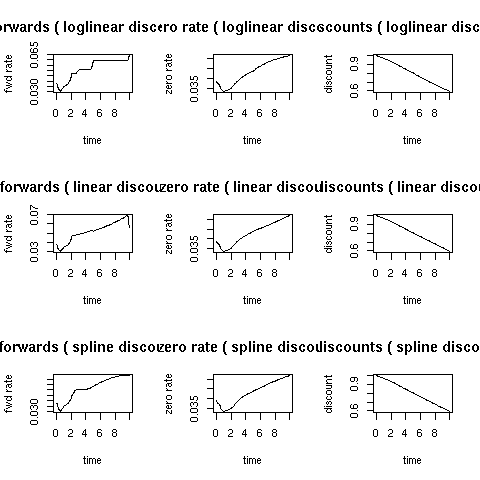
An example for DiscountCurves

> example(DiscountCurve)

DscntC> savepar <- par(mfrow = c(3, 3))

DscntC> params <- list(tradeDate = c(2, 15, 2002), settleDate = c(2,
    19, 2002), dt = 0.25, interpWhat = "discount", interpHow = "loglinear")

DscntC> tsQuotes <- list(d1w = 0.0382, d1m = 0.0372, fut1 = 96.2875,
    fut2 = 96.7875, fut3 = 96.9875, fut4 = 96.6875, fut5 = 96.4875,
    fut6 = 96.3875, fut7 = 96.2875, fut8 = 96.0875, s3y = 0.0398,
    s5y = 0.0443, s10y = 0.05165, s15y = 0.055175)

DscntC> times <- seq(0, 10, 0.1)

DscntC> curves <- DiscountCurve(params, tsQuotes, times)

DscntC> plot(curves, setpar = FALSE)

DscntC> params$interpHow = "linear"

DscntC> curves <- DiscountCurve(params, tsQuotes, times)

DscntC> plot(curves, setpar = FALSE)

DscntC> params$interpHow = "spline"

DscntC> curves <- DiscountCurve(params, tsQuotes, times)

DscntC> plot(curves, setpar = FALSE)

DscntC> par(savepar)

Download

Alternatively, you can also get RQuantLib from a Comprehensive R Archive Network (CRAN) node in the src/contrib directory.

Lastly, RQuantLib sources are now hosted at R-Forge; please see the RQuantLib page at R-Forge for an overview and access to the SVN archive. Potential contributors are welcome: please register at R-Forge and contact me if you want to contribute.

Installation on Unix

For Debian users, this is as simple as saying apt-get install libquantlib0 libquantlib-dev. Others will have to compile QuantLib, see the QuantLib site.

Generally, for Linux or Unix users, the usual R CMD INSTALL RQuantLib should work from outside R, as should a call to install.packages(). At least, it does on my Debian Linux system.

Feedback and comments are of course welcome in general, and in particular on the installation.

Installation on Windows

Changelog

2008-01-01  Dirk Eddelbuettel  

	* DESCRIPTION: Release 0.2.8, updated for QL 0.9.0

	* R/option.R: For BinaryOption, added new arguments 'binType' and
	  'excType' to select the type of Binary (cash, asset or gap) and
	  exercise (european or american).

	* RcppSrc/Rcpp.cpp,src/*cpp: Added const char* casts for Rprintf
	* src/BinaryOptions.cpp: Support new binType and excType arguments
	* src/*cpp: Generally updated for QL 0.9.0 changes
	* src/discount.cpp: New boolean variable flatQuotes
	
	* man/{BinaryOption,DiscountCurve}.Rd: Updated for new arguments

	* inst/unitTests: Added unit testing using the RUnit package

2007-07-01  Dirk Eddelbuettel  

	* DESCRIPTION: Release 0.2.7, updated for QL 0.8.1
	
	* configure.in: Require QuantLib 0.8.1, and Boost 1.34.0

2007-06-30  Dominick Samperi  

	* src/bermudan.cpp, src/curves.cpp: Updated for QL 0.8.1

2007-02-25  Dirk Eddelbuettel  

	* DESCRIPTION: Relase 0.2.5 updated for Quantlib 0.4.0

	* configure.in: Require Quantlib 0.4.0

2007-02-24  Dominick Samperi  

	* src/bermudan.cpp: Several updates for Quantlib 0.4.0

2006-11-10  Dirk Eddelbuettel  

	* man/*.Rd: Updates to default method docs suggested by Kurt Hornik
	
2006-11-06  Dirk Eddelbuettel  

	* DESCRIPTION: Release 0.2.5 updated for QuantLib 0.3.14

	* src/*.cpp:  Several minor changes for class renaming and
	  interface changes on the QuantLib side of things

2006-08-14  Dirk Eddelbuettel  

	* DESCRIPTION: Release 0.2.4 updated for QuantLib 0.3.13; this
	  required some changes in the fixed-income functions

	* configure.in: Tests for QuantLib version 0.3.13

	* tests/RQuantLib.R: Added the beginnings of unit-tests
	* tests/RQuantLib.Rout.save: Control output for unit tests

2006-07-23  Dirk Eddelbuettel  

	* DESCRIPTION: Release 0.2.3 using the new RcppTemplate version 4.2
	 
	* src/*: RcppTemplate is now used for all R/C++ interfaces
	  features from the new RcppTemplate

2006-03-30  Dirk Eddelbuettel  

	* Release 0.2.2 once more with thanks to Dominick

2006-03-23  Dominick Samperi  

	* configure.in, configure.win,
	  inst/lib/Makefile, inst/lib/Makefile.win,
	  src/Makefile, src/Makefile.win,
	  cleanup: modified to support use of RcppTemplate V2.2.
          RQuantLib shared library (or DLL) is created by linking
          against RcppSrc/libRcpp.a.
	  Tested against QuantLib 0.3.12.

	* Rcpp.{cpp,hpp}: added latest versions from RcppTemplate package.

2006-01-10  Dirk Eddelbuettel  

	* Release 0.2.1 with thanks to Dominick

2006-01-10  Dominick Samperi 

	* man/DiscountCurve.Rd: Fixed typo and commented out rates
	  needing to be fractions in fixed formating in DiscountCurve example

	* src/Rcpp.{hpp,cpp},src/{curves,discount,bermudan}.cpp:
	  modified to throw exceptions instead of calling R's error() function.
2005-10-27  Dominick Samperi 

	* src/Rcpp.{hpp,cpp}: Some minor adjustments. Moved matrix and
	  vector indexing into header file.
	
	* src/rquantlib.hpp: Added ifdef to protect against multiple includes.

2005-10-26  Dirk Eddelbuettel  

	* Preparing release 0.2.0 regrouping the numerous changes --
	  contributed mostly by Dominick -- since the 0.1.13 release

2005-10-13  Dominick Samperi 

	* src/Rcpp.{hpp,cpp}: Improved error messages

2005-10-08  Dominick Samperi 

	* src/Rcpp.cpp: Implemented Rcpp, R/C++ interface classes, and
	  modified discount.cpp and bermudan.cpp to use it.

	* src/Rcpp.hpp: Header files for latter.
	
2005-10-03  Dominick Samperi 

	* inst/Boost-License.txt, inst/QuantLib-License.txt: License files
	  for Boost and QuantLib.

	* Windows is now supported using a binary package that does not
	  require the user to install a compiler, Boost, or QuantLib. Had
	  to add Makefile.win, configure.win, etc.
	
	* R/discount.R: new DiscountCurve function that constructs the
	  spot term structure of interest rates based on
	  market observables like
	  deposit rates, futures prices, FRA rates, and swap rates. Supports
	  the fitting of discount factors, forward rates, or zero coupon
	  rates, using linear, log-linear, and cubic spline interpolation.

	* man/DiscountCurve.Rd: man page for DiscountCurve.
	
	* R/bermudan.R: new function that prices a Bermudan swaption
	  using a choice of four models: G2 analytic, Hull-White analytic,
	  Hull-White tree, and Black-Karasinski tree.

	* man/BermudanSwaption.Rd: man page for BermudanSwaption.
	
	* src/curves.cpp: utility code for curve construction.

	* src/discount.cpp: implements DiscountCurve.

	* src/bermudan.cpp: implements BermudanSwaption.

	* src/utils.cpp: added utility functions to simplify communication
	  with R.

	* src/rquantlib.hpp: contains prototypes for utility functions and
	  new definitions for Windows.

	* Changed: suffix .cc to .cpp, and .h to .hpp.
	
2005-09-16  Dirk Eddelbuettel  

	* demo/OptionSurfaces.R: added demo with OpenGL visualizations
	  of option analytics, requires rgl package
	  [ Update: not released as rgl crashes on some platforms ]

2005-08-06  Dirk Eddelbuettel  

	* Release 0.1.13 matching the new QuantLib 0.3.10 release

	* Implied volatilies are back!
	  With gcc/g++ 4.0, the segmentation fault that I was seeing
	  on implied volatility using gcc/g++ 3.3 (but which others did
	  not see with gcc/g++ 3.2) has disappeared, so the
	  corresponding code has been reactivated.
	* BinaryOptionImpliedVolatility() is also back

	* src/*.cc, R/*.R: Removed a lot of commented-out code

2005-04-26  Dirk Eddelbuettel  

	* Release 0.1.12 matching the upcoming QuantLib 0.3.9 release
	
	* configure.in: Test for QuantLib>= 0.3.8

	* src/*.cc: Several changes for QuantLib 0.3.9:
	  - use Handle<...> instead of RelinkableHandle<...>
	  - use YieldTermStructure instead of TermStructure
	  - use today + length instead of today.plusDays

2004-12-27  Dirk Eddelbuettel  

	* Release 0.1.11 matching the new QuantLib 0.3.8 release

	* configure.in: Added tests for Boost headers, with thanks and
	  a nod to QuantLib for the actual autoconf code

	* src/{barrier_binary.cc,implieds.cc,vanilla.cc}: Option type
	  'Straddle' now unsupported, hence commented out
	* man/*.Rd: Similarly removed reference to straddle from docs
	
	* src/{barrier_binary.cc,implieds.cc,utils.cc,vanilla.cc}:
	  Renamed BlackScholesStochasticProcess to BlackScholesProcess

	* src/vanilla.cc: Changed Handle to boost::shared_ptr
	
2004-09-12  Dirk Eddelbuettel  

	* Release 0.1.10

	* Switched to using Boost library as per QuantLin 0.3.7

        * AmericanOption now uses the Barone-Adesi-Whaley approximation
	
	* Implied volatility for both European and American options
	  currently segfaults when called from R, though the code itself
	  works as standalon. The code also works from R when the implied
	  calculation call is skipped. Something is corrupting memory
	  somewhere. For now, we return NA for either function.

2004-08-06  Dirk Eddelbuettel  

	* DESCRIPTION: Added SystemRequirements for QuantLib

2004-05-26  Dirk Eddelbuettel  

	* Release 0.1.9

	* man/EuropeanOption.Rd: Added corrections for the issues raised
	  by Ajay Shah in the Debian bug report #249240

	* man/{AmericanOption,BarrierOption,BinaryOption}.Rd: Idem

2004-04-05  Dirk Eddelbuettel  

	* Release 0.1.8

	* src/{barrier_binary,implieds,utils,vanilla}.cc: Updated to the
	  new QuantLib 0.3.5 pricer framework.  This currently implies
	  that options priced using the binomial engines do not have
	  Greeks; this should be addressed in a future QuantLib release.

	* man/{BarrierOption,AmericanOption}.Rd: Note that Greeks are
	  currently unavailable with binary pricers
	 

2003-11-28  Dirk Eddelbuettel  

	* Release 0.1.7

	* src/barrier_binary.cc:
	  -- split off from RQuantLib.cc
	  -- added three more greeks to Barrier Option
	  -- reflected small change in QuantLib types for Barrier Options

	* src/implieds.cc
	  -- split off from RQuantLib.cc
	  -- rewritten functions for implied volatility on European and
	     American options using new QuantLib framework
	
	* src/utils.cc
	  -- split off from RQuantLib.cc

	* src/vanilla.cc
	  -- rump of RQuantLib.cc, renamed
	
2003-07-31  Dirk Eddelbuettel  

	* Release 0.1.6

	* man/{EuropeanOption,ImpliedVolatility}: Two small corrections
	  to argument call mismatches found by R CMD check

2003-05-31  Dirk Eddelbuettel  

	* Release 0.1.5

	* R/{option,implied}.R: generic/method consistency improved
	  following heads-up, and subsequent help, from BDR. Thanks!
	
2003-03-25  Dirk Eddelbuettel  

	* Release 0.1.4
	
	* data/:  Removed empty directory as suggested by Kurt

	* configure.in: Several additions:
	  - test for g++>= 3.0, kindly provided by Kurt
	  - test for QuantLib>= 0.3, along the same lines
	  - converted from autoconf 2.13 to 2.50
	
	* cleanup: Remove temp dir created by autoconf

2003-02-05  Dirk Eddelbuettel  

	* Release 0.1.3

	* R/*.R: Added PACKAGE="RQuantLib" to .Call() as suggested by Kurt

	* DESCRIPTION: Removed QuantLib from Depends as requested by Kurt,
  	  and added explanation to Description

2002-11-13  Dirk Eddelbuettel  

	* Release 0.1.2

	* Minor correction to EuropeanOptionArrays manual page indexing

2002-11-11  Dirk Eddelbuettel  

	* Release 0.1.1

	* Added barrier option

	* Minor corrections and completions to documentation
	  
2002-02-25  Dirk Eddelbuettel  

	* Initial 0.1.0 release

Copyright

RQuantLib is Copyright(c) 2002 - 2008 by Dirk Eddelbuettel, and Copyright(c) 2005 - 2008 by Dominick Samperi.

This program is free software; you can redistribute it and/or modify it under the terms of the GNU General Public License as published by the Free Software Foundation; either version 2 of the License, or (at your option) any later version. There is NO warranty whatsoever. This package is released under the GNU General Public License

GNU R is released under the same terms, the GNU General Public License.

QuantLib is released under the QuantLib license, a modified BSD license which is compatible with the GPL, see Quantlib's license and copyrights page.

Last modified: Sat Jan 5 09:41:26 CST 2008