Rcpp attributes: A simple example 'making pi'
We introduced Rcpp 0.10.0 with a number of very nice new features a few days ago, and the activity on the rcpp-devel mailing list has been pretty responsive which is awesome.But because few things beat a nice example, this post tries to build some more excitement. We will illustrate how Rcpp attributes makes it really easy to add C++ code to R session, and that that code is as easy to grasp as R code.
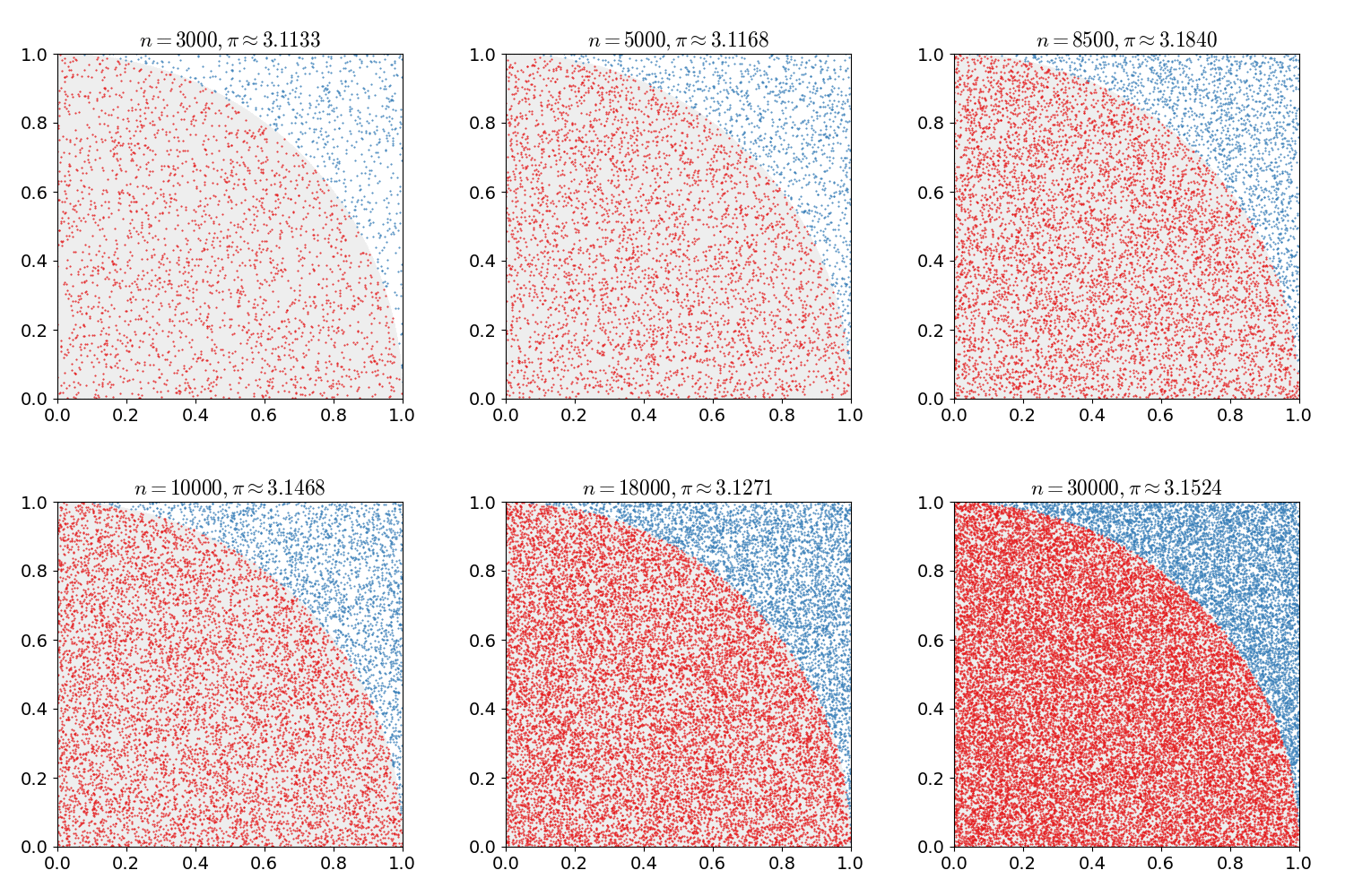
Our motivating example is everybody's favourite introduction to Monte Carlo simulation: estimating π. A common method uses the fact
the unit circle has a surface area equal to π. We draw two uniform random numbers x and y, each between zero
and one. We then check for the distance of the corresponding point (x,y) relative to the origin. If less than one (or equal),
it is in the circle (or on it); if more than one it is outside. As the first quadrant is a quarter of a square of area one, the area of
the whole circle is π -- so our first quadrant approximates π over four. The following figure, kindly borrowed from Wikipedia
with full attribution and credit, illustrates this:

Now, a vectorized version (drawing N such pairs at once) of this approach is provided by the following R function.
piR <- function(N) {
    x <- runif(N)
    y <- runif(N)
    d <- sqrt(x^2 + y^2)
    return(4 * sum(d < 1.0) / N)
}
And in C++ we can write almost exactly the same function thanks the Rcpp sugar vectorisation available via Rcpp:
Sure, there are small differences: C++ is statically typed, R is not. We need one include file for declaration, and we need one instantiation of the#include <Rcpp.h> using namespace Rcpp; // [[Rcpp::export]] double piSugar(const int N) { RNGScope scope; // ensure RNG gets set/reset NumericVector x = runif(N); NumericVector y = runif(N); NumericVector d = sqrt(x*x + y*y); return 4.0 * sum(d < 1.0) / N; }
RNGScope object to ensure random number draws remain coordinated between the calling R process and the C++ function
calling into its (compiled C-code based) random number generators. That way we even get the exact same draws for the same seed.
But the basic approach is identical: draw a vector x and vector y, compute the distance to the origin and then
obtain the proportion within the unit circle -- which we scale by four. Same idea, same vectorised implementation in C++.
But the real key here is the one short line with the [[Rcpp::export]] attribute. This is all it takes (along with
sourceCpp() from Rcpp 0.10.0) to get the C++ code into R.
The full example (which assumes the C++ file is saved as piSugar.cpp in the same directory) is now:
and it does a few things: set up the R function, source the C++ function (and presto: we have a callable C++ function just like that), compute two simulations given the same seed and ensure they are in fact identical -- and proceed to compare the timing in a benchmarking exercise. That last aspect is not even that important -- we end up being almost-but-not-quite twice as fast on my machine for different values of#!/usr/bin/r library(Rcpp) library(rbenchmark) piR <- function(N) { x <- runif(N) y <- runif(N) d <- sqrt(x^2 + y^2) return(4 * sum(d < 1.0) / N) } sourceCpp("piSugar.cpp") N <- 1e6 set.seed(42) resR <- piR(N) set.seed(42) resCpp <- piSugar(N) ## important: check results are identical with RNG seeded stopifnot(identical(resR, resCpp)) res <- benchmark(piR(N), piSugar(N), order="relative") print(res[,1:4])
N.
The real takeaway here is the ease with which we can get a C++ function into R --- and the new process completely takes care of passing parameters in, results out, and does the compilation, linking and loading.
More details about Rcpp attributes are in the new vignette. Now enjoy the π.
Update:One somewhat bad typo fixed.
Update:Corrected one background tag.