Rcpp attributes: Even easier integration of GSL code into R
Following the Rcpp 0.10.0 release, I had written about simulating pi easily by using the wonderful new Rcpp Attributes feature. Now with Rcpp 0.10.1 released a good week ago, it is time to look at how Rcpp Attributes can help with external libraries. As this posts aims to show, it is a breeze!One key aspect is the use of the plugins for the inline package. They provide something akin to a callback mechanism so that compilation and linking steps can be informed about header and library locations and names. We are going to illustrate this with an example from GNU Scientific Library (GSL). The example I picked uses B-Spline estimation from the GSL. This is a little redundant as R has its own spline routines and package, but serves well as a simple illustration---and, by reproducing an existing example, followed an established path. So we will look at Section 39.7 of the GSL manual which has a complete example as a standalone C program, generating both the data and the fit via cubic B-splines.
We can decompose this two parts: data generation, and fitting. We will provide one function each, and then use both from R. These two function will follow the aforementioned example from Section 39.7 somewhat closely.
We start with the first function to generate the data.
We include a few header files, define (in what is common for C programs) a few constants and then define a single function// [[Rcpp::depends(RcppGSL)]] #include <RcppGSL.h> #include <gsl/gsl_bspline.h> #include <gsl/gsl_multifit.h> #include <gsl/gsl_rng.h> #include <gsl/gsl_randist.h> #include <gsl/gsl_statistics.h> const int N = 200; // number of data points to fit const int NCOEFFS = 12; // number of fit coefficients */ const int NBREAK = (NCOEFFS - 2); // nbreak = ncoeffs + 2 - k = ncoeffs - 2 since k = 4 */ // [[Rcpp::export]] Rcpp::List genData() { const size_t n = N; size_t i; double dy; gsl_rng *r; RcppGSL::vector<double> w(n), x(n), y(n); gsl_rng_env_setup(); r = gsl_rng_alloc(gsl_rng_default); //printf("#m=0,S=0\n"); /* this is the data to be fitted */ for (i = 0; i < n; ++i) { double sigma; double xi = (15.0 / (N - 1)) * i; double yi = cos(xi) * exp(-0.1 * xi); sigma = 0.1 * yi; dy = gsl_ran_gaussian(r, sigma); yi += dy; gsl_vector_set(x, i, xi); gsl_vector_set(y, i, yi); gsl_vector_set(w, i, 1.0 / (sigma * sigma)); //printf("%f %f\n", xi, yi); } Rcpp::DataFrame res = Rcpp::DataFrame::create(Rcpp::Named("x") = x, Rcpp::Named("y") = y, Rcpp::Named("w") = w); x.free(); y.free(); w.free(); gsl_rng_free(r); return(res); }
genData() which returns and Rcpp::List as a list object to R. A primary importance here are the two attributes:
one to declare a dependence on the RcppGSL package, and one to declare the
export of the data generator function. That is all it takes! The plugin of the
RcppGSL will provide information about the headers and library, and Rcpp
Attributes will do the rest.
The core of the function is fairly self-explanatory, and closely follows the
original example. Space gets
allocated, the RNG is setup and a simple functional form generates some data plus noise (see below). In the original, the data is written to
the standard output; here we return it to R as three columns in a data.frame object familiar to R users. We then free the GSL
vectors; this manual step is needed as they are implemented as C vectors which do not have a destructor.
Next, we can turn the fitting function.
// [[Rcpp::export]]
Rcpp::List fitData(Rcpp::DataFrame ds) {

    const size_t ncoeffs = NCOEFFS;
    const size_t nbreak = NBREAK;

    const size_t n = N;
    size_t i, j;

    Rcpp::DataFrame D(ds);              // construct the data.frame object
    RcppGSL::vector<double> y = D["y"]; // access columns by name,
    RcppGSL::vector<double> x = D["x"]; // assigning to GSL vectors
    RcppGSL::vector<double> w = D["w"];

    gsl_bspline_workspace *bw;
    gsl_vector *B;
    gsl_vector *c;
    gsl_matrix *X, *cov;
    gsl_multifit_linear_workspace *mw;
    double chisq, Rsq, dof, tss;

    bw = gsl_bspline_alloc(4, nbreak);      // allocate a cubic bspline workspace (k = 4)
    B = gsl_vector_alloc(ncoeffs);

    X = gsl_matrix_alloc(n, ncoeffs);
    c = gsl_vector_alloc(ncoeffs);
    cov = gsl_matrix_alloc(ncoeffs, ncoeffs);
    mw = gsl_multifit_linear_alloc(n, ncoeffs);

    gsl_bspline_knots_uniform(0.0, 15.0, bw);   // use uniform breakpoints on [0, 15]

    for (i = 0; i < n; ++i) {                   // construct the fit matrix X
        double xi = gsl_vector_get(x, i);

        gsl_bspline_eval(xi, B, bw);            // compute B_j(xi) for all j

        for (j = 0; j < ncoeffs; ++j) {         // fill in row i of X
            double Bj = gsl_vector_get(B, j);
            gsl_matrix_set(X, i, j, Bj);
        }
    }

    gsl_multifit_wlinear(X, w, y, c, cov, &chisq, mw);  // do the fit

    dof = n - ncoeffs;
    tss = gsl_stats_wtss(w->data, 1, y->data, 1, y->size);
    Rsq = 1.0 - chisq / tss;

    Rcpp::NumericVector FX(151), FY(151);       // output the smoothed curve
    double xi, yi, yerr;
    for (xi = 0.0, i=0; xi < 15.0; xi += 0.1, i++) {
        gsl_bspline_eval(xi, B, bw);
        gsl_multifit_linear_est(B, c, cov, &yi, &yerr);
        FX[i] = xi;
        FY[i] = yi;
    }

    Rcpp::List res =
      Rcpp::List::create(Rcpp::Named("X")=FX,
                         Rcpp::Named("Y")=FY,
                         Rcpp::Named("chisqdof")=Rcpp::wrap(chisq/dof),
                         Rcpp::Named("rsq")=Rcpp::wrap(Rsq));

    gsl_bspline_free(bw);
    gsl_vector_free(B);
    gsl_matrix_free(X);
    gsl_vector_free(c);
    gsl_matrix_free(cov);
    gsl_multifit_linear_free(mw);

    y.free();
    x.free();
    w.free();

    return(res);
}
The second function closely follows the second part of the GSL example and, given the input data, fits the output data. Data structures are setup, the spline basis is created, data is fit and then the fit is evaluated at a number of points. These two vectors are returned along with two goodness of fit measures.
We only need to load the Rcpp package and source a file containing the two snippets shown above, and we are ready to deploy this:
library(Rcpp)
sourceCpp("bSpline.cpp")                # compile two functions
dat <- genData()                        # generate the data
fit <- fitData(dat)                     # fit the model, returns matrix and gof measures
And with that, we generate a chart such as
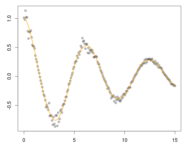
via a simple four lines, or as much as it took to create the C++ functions, generate the data and fit it!
op <- par(mar=c(3,3,1,1))
plot(dat[,"x"], dat[,"y"], pch=19, col="#00000044")
lines(fit[[1]], fit[[2]], col="orange", lwd=2)
par(op)
The RcppArmadillo and RcppEigen package support plugin use in the same way. Add an attribute to export a function, and an attribute for the depends -- and you're done. Extending R with (potentially much faster) C++ code has never been easier, and opens a whole new set of doors.