Updated overbought/oversold plot function
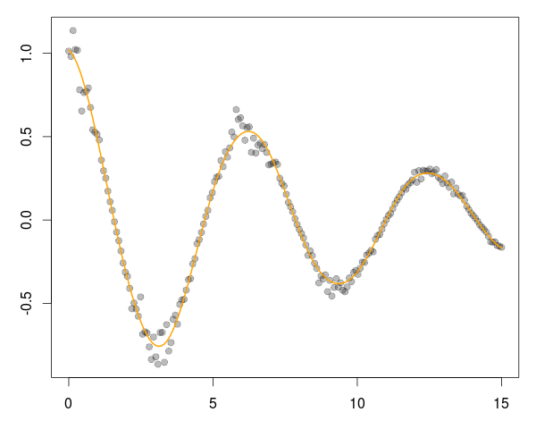
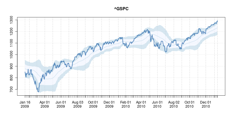
A good six years ago I blogged about plotOBOS() which charts a moving average (from one of several available variants) along with shaded standard deviation bands. That post has a bit more background on the why/how and motivation, but as a teaser here is the resulting chart of the SP500 index (with ticker ^GSCP):
The code uses a few standard finance packages for R (with most of them maintained by Joshua Ulrich given that Jeff Ryan, who co-wrote chunks of these, is effectively retired from public life). Among these, xts had a recent release reflecting changes which occurred during the four (!!) years since the previous release, and covering at least two GSoC projects. With that came subtle API changes: something we all generally try to avoid but which is at times the only way forward. In this case, the shading code I used (via polygon() from base R) no longer cooperated with the beefed-up functionality of plot.xts(). Luckily, Ross Bennett incorporated that same functionality into a new function addPolygon --- which even credits this same post of mine.
With that, the updated code becomes
## plotOBOS -- displaying overbough/oversold as eg in Bespoke's plots
##
## Copyright (C) 2010 - 2017 Dirk Eddelbuettel
##
## This is free software: you can redistribute it and/or modify it
## under the terms of the GNU General Public License as published by
## the Free Software Foundation, either version 2 of the License, or
## (at your option) any later version.
suppressMessages(library(quantmod)) # for getSymbols(), brings in xts too
suppressMessages(library(TTR)) # for various moving averages
plotOBOS <- function(symbol, n=50, type=c("sma", "ema", "zlema"),
years=1, blue=TRUE, current=TRUE, title=symbol,
ticks=TRUE, axes=TRUE) {
today <- Sys.Date()
if (class(symbol) == "character") {
X <- getSymbols(symbol, from=format(today-365*years-2*n), auto.assign=FALSE)
x <- X[,6] # use Adjusted
} else if (inherits(symbol, "zoo")) {
x <- X <- as.xts(symbol)
current <- FALSE # don't expand the supplied data
}
n <- min(nrow(x)/3, 50) # as we may not have 50 days
sub <- ""
if (current) {
xx <- getQuote(symbol)
xt <- xts(xx$Last, order.by=as.Date(xx$`Trade Time`))
colnames(xt) <- paste(symbol, "Adjusted", sep=".")
x <- rbind(x, xt)
sub <- paste("Last price: ", xx$Last, " at ",
format(as.POSIXct(xx$`Trade Time`), "%H:%M"), sep="")
}
type <- match.arg(type)
xd <- switch(type, # compute xd as the central location via selected MA smoother
sma = SMA(x,n),
ema = EMA(x,n),
zlema = ZLEMA(x,n))
xv <- runSD(x, n) # compute xv as the rolling volatility
strt <- paste(format(today-365*years), "::", sep="")
x <- x[strt] # subset plotting range using xts' nice functionality
xd <- xd[strt]
xv <- xv[strt]
xyd <- xy.coords(.index(xd),xd[,1]) # xy coordinates for direct plot commands
xyv <- xy.coords(.index(xv),xv[,1])
n <- length(xyd$x)
xx <- xyd$x[c(1,1:n,n:1)] # for polygon(): from first point to last and back
if (blue) {
blues5 <- c("#EFF3FF", "#BDD7E7", "#6BAED6", "#3182BD", "#08519C") # cf brewer.pal(5, "Blues")
fairlylight <<- rgb(189/255, 215/255, 231/255, alpha=0.625) # aka blues5[2]
verylight <<- rgb(239/255, 243/255, 255/255, alpha=0.625) # aka blues5[1]
dark <<- rgb(8/255, 81/255, 156/255, alpha=0.625) # aka blues5[5]
## buglet in xts 0.10-0 requires the <<- here
} else {
fairlylight <<- rgb(204/255, 204/255, 204/255, alpha=0.5) # two suitable grays, alpha-blending at 50%
verylight <<- rgb(242/255, 242/255, 242/255, alpha=0.5)
dark <<- 'black'
}
plot(x, ylim=range(range(x, xd+2*xv, xd-2*xv, na.rm=TRUE)), main=title, sub=sub,
major.ticks=ticks, minor.ticks=ticks, axes=axes) # basic xts plot setup
addPolygon(xts(cbind(xyd$y+xyv$y, xyd$y+2*xyv$y), order.by=index(x)), on=1, col=fairlylight) # upper
addPolygon(xts(cbind(xyd$y-xyv$y, xyd$y+1*xyv$y), order.by=index(x)), on=1, col=verylight) # center
addPolygon(xts(cbind(xyd$y-xyv$y, xyd$y-2*xyv$y), order.by=index(x)), on=1, col=fairlylight) # lower
lines(xd, lwd=2, col=fairlylight) # central smooted location
lines(x, lwd=3, col=dark) # actual price, thicker
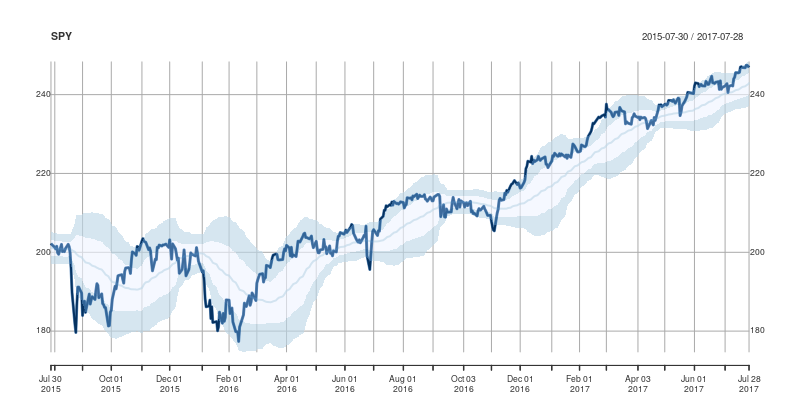
}and the main change are the three calls to addPolygon. To illustrate, we call plotOBOS("SPY", years=2) with an updated plot of the ETF representing the SP500 over the last two years:
Comments and further enhancements welcome!
This post by Dirk Eddelbuettel originated on his Thinking inside the box blog. Please report excessive re-aggregation in third-party for-profit settings.